WMH segmentation challenge
Hugo Kuijf – UMC Utrecht – December 2022Note: the challenge is closed. All training, test, and manual annotation data can be downloaded here: https://doi.org/10.34894/AECRSD.
Table of Contents
Introduction
The White Matter Hyperintensity (WMH) Segmentation Challenge was a biomedical challenge, organized in association with MICCAI 2017 in Quebec. It was active in 2017 – 2022, after which all training and test data was released.
This document contains all information provided at the challenge website: https://wmh.isi.uu.nl/ as of December 2022. Information may be outdated and links might not work.
 Aim
Aim
The purpose of this challenge is to directly compare methods for the automatic segmentation of White Matter Hyperintensities (WMH) of presumed vascular origin.
Outline
To participate in the challenge, interested teams can register on this website. After registration, training data can be downloaded. This data consists of 60 sets of brain MR images (T1 and FLAIR) with manual annotations of WMH (binary masks) from three different institutes / scanners. Manual annotations have been made by experts in WMH scoring.
Participants can train their methods on the available data and submit the resulting method for evaluation by the organizers. A brief description (1-2 pages) of the method should be included. Test data will not be released, but consists of 110 sets of brain MR images from five different scanners (of which three are also in the training data).
Reference
Initial results of this challenge have been published by IEEE Transactions on Medical Imaging. Please cite this paper in scientific output resulting from your participation: Kuijf, H. J., et al. “Standardized Assessment of Automatic Segmentation of White Matter Hyperintensities; Results of the WMH Segmentation Challenge.” IEEE transactions on medical imaging (2019).
MICCAI 2017
The kick-off meeting of this challenge was organized at MICCAI 2017 in Quebec, Canada. Initially, twenty teams participated and presented their method. The challenge remained open and is ongoing since then. These slides were presented during the challenge session at MICCAI 2017.
These presentations can be used under the Creative Commons Attribution 4.0 International License.
Details
Task
The segmentation of white matter hyperintensities of presumed vascular origin on brain MR images.
Background
Small vessel disease plays a crucial role in stroke, dementia, and ageing1. White matter hyperintensities (WMH) of vascular origin are one of the main consequences of small vessel disease and well visible on brain MR images2. Quantification of WMH volume, location, and shape is of key importance in clinical research studies and likely to find its way into clinical practice; supporting diagnosis, prognosis, and monitoring of treatment for dementia and other neurodegenerative diseases. It has been noted that visual rating of WMH has important limitations3 and hence a more detailed segmentation of WMH is preferred. Various automated WMH segmentation techniques have been developed, to provide quantitative measurements and replace time-consuming, observer-dependent delineation procedures.
A review on automated WMH segmentation techniques revealed a key issue: it is hard to compare various techniques3. Each segmentation technique is evaluated on a different ground truth (different number of subjects, different experts, different protocols) and using different evaluation criteria.
This challenge aims to directly compare automated WMH segmentation techniques. The output will be a ranking of techniques that robustly and accurately segment WMH across different scanner platforms and different subject groups.
Method
Participants will containerize their algorithms with Docker and submit these to the organizers. Detailed instructions and easy-to-follow examples are provided and, if needed, the organizers will help with containerization. The organizers will run the techniques on the test data. This guarantees that the test data remains secret and cannot be included in the training procedure of the techniques.
The container / Docker infrastructure guarantees standardized testing in the coming years, and is supported by the UMC Utrecht. The main organizer and the UMC Utrecht agree to commit themselves to future support of this challenge.
Results
The organizers will evaluate all methods according to the evaluation criteria. The results will be published on this website, showing the overall results in a table and detailed results on a separate page per method.
Terms of participation
The WMH Segmentation Challenge is organized in the spirit of cooperative scientific progress. We do not claim any ownership or right to the methods, but we require anyone to respect the rules below. The following rules apply to those who register a team and/or download the data:
- The downloaded data sets, associated reference standard, or any data derived from these data sets, may not be given or redistributed under any circumstances to persons not belonging to the registered team.
- All information entered when registering a team, including the name of the contact person, the affiliation (institute, organization or company the team’s contact person works for) and the e-mail address must be complete and correct. Anonymous or incomplete registration is not allowed. If you wish to submit anonymously, for example because you want to submit your results to a journal or conference that requires anonymous submission, please contact the organizers first.
- The data provided may only be used for preparing an entry to be submitted to this challenge. The data may not be used for other purposes in scientific studies and may not be used to train or develop other algorithms, including but not limited to algorithms used in commercial products, without prior participation in the challenge and approval by the organizers.
- Results of your submission will only be published on the website when a document describing the method is provided.
- If a commercial system is evaluated no method description is necessary, but the system has to be publicly available and the exact name and version number have to be provided.
- The organizers of the challenge will check the method description before your results will be published on the website.
- If the results of algorithms in this challenge are to be used in scientific publications (e.g. journal publications, conference papers, technical reports, presentations at conferences and meetings) you must make an appropriate citation to : Kuijf, H. J., et al. “Standardized Assessment of Automatic Segmentation of White Matter Hyperintensities; Results of the WMH Segmentation Challenge.” IEEE transactions on medical imaging (2019).
- Evaluation of registration results uploaded to this website will be made publicly available on this website (Results section), and by submitting results, you grant us permission to publish our evaluation. Participating teams maintain full ownership and rights to their method.
- Teams must notify the organizers of this challenge about any publication that is (partly) based on the results data published on this website, in order for us to maintain a list of publications associated with the challenge.
This agreement needs to be signed and mailed, to activate your registration and get access to the data.
References
Data
Image data used in this challenge were acquired from five different scanners from three different vendors in three different hospitals in the Netherlands and Singapore. For each subject, a 3D T1-weighted image and a 2D multi-slice FLAIR image are provided. The manual reference standard is defined on the FLAIR image.
Details
|
Institute |
Scanner |
#training |
#test |
|
UMC Utrecht |
3 T Philips Achieva |
20 |
30 |
|
NUHS Singapore |
3 T Siemens TrioTim |
20 |
30 |
|
VU Amsterdam |
3 T GE Signa HDxt |
20 |
30 |
|
3 T Philips Ingenuity |
0 |
10 |
|
|
1.5 T GE Signa HDxt |
0 |
10 |
For each subject, the following files are provided:
|
File |
Details |
|
/orig/3DT1.nii.gz |
The original 3D T1 image, with the face removed. |
|
/orig/3DT1_mask.nii.gz |
Binary mask used to remove the face. |
|
/orig/FLAIR.nii.gz |
The original FLAIR image. This image is used to manually delineate the WMH and participants should provide the results in this image space. |
|
/orig/reg_3DT1_to_FLAIR.txt |
Transformation parameters used to align the 3D T1 image with the FLAIR image. Participants can use this to do the transformation themselves, in case they use the 3D T1 for processing. Results will be evaluated in the FLAIR space. Call: transformix -in IMAGE.EXT -out /output -tp /orig/reg_3DT1_to_T2_FLAIR.txt |
|
/orig/T1.nii.gz |
The 3D T1 image aligned with the FLAIR image. |
|
/pre/3DT1.nii.gz |
Bias field corrected 3D T1 image. |
|
/pre/FLAIR.nii.gz |
Bias field corrected FLAIR image. |
|
/pre/T1.nii.gz |
Bias field corrected T1 image, aligned with FLAIR. |
|
/wmh.nii.gz |
Manual reference standard, only available for training data. |
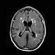
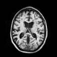
Example images
|
orig/3DT1 |
orig/3DT1 mask |
orig/FLAIR |
orig/T1 |
|
pre/3DT1 |
pre/FLAIR |
pre/T1 |
WMH |

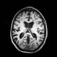
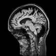
Top row shows all images present in the folder orig. Bottom row shows the pre-processed images and the manual WMH segmentation.
Folder: orig
This folder contains the original images, anonimized and having the face removed. The mask used to remove the face from the 3D T1 images is provided. The 3D T1 image has been aligned with the FLAIR image using elastix 4.8 with the following parameter file: elastix parameter file for the WMH Segmentation Challenge.
Folder: pre
All images were pre-processed with SPM12 r6685 to correct bias field inhomogeneities.
Manual reference standard
This file is only provided for the training data and it contains the following three labels:
0. Background
1. White matter hyperintensities
2. Other pathology
The objective of this challenge is to automatically segment WMH. Because we do not require methods to identify all other types of pathology, we provide a rough mask for them that will be ignored during evaluation.
Additional data
Participants are allowed to use additional data to train their method. This must be mentioned in the description that is submitted with the method. We encourage participants to use open data or make the additional data open access.
Manual reference standard
Training data is accompanied by the manual reference standard, containing the following three labels:
0. Background
1. White matter hyperintensities
2. Other pathology
The objective of this challenge is to automatically segment WMH (label 0 vs 1). Because we do not require methods to identify all other types of pathology, we provide a rough mask (label 2) for them that is ignored during evaluation.
Rating criteria
WMH and other pathology were manually segmented according to the STandards for ReportIng Vascular changes on nEuroimaging (STRIVE). One expert observer (O1) segmented all images using a contour drawing technique, delineating the outline of all WMH. This observer O1 has extensive prior experience with the manual segmentation of WMH and has segmented 500+ cases. A second expert observer (O2) performed extensive peer review on all manual delineations. In case of mistakes, errors, or delineations that were not according to the STRIVE standards, O1 corrected the segmentation. Hence, the provided reference standard is the corrected segmentation of O1, after peer review by O2.
Binary masks
The contours were converted to binary masks, including all voxels whose volume >50% was included within the manually drawn contour. Background received label 0 and WMH label 1.
Other pathology was converted to binary masks as well, receiving label 2. These masks were dilated by 1 pixel in-plane (with a 3x3x1 kernel). In case of overlap between labels 1 and 2, label 1 was assigned.
Inter observer agreement
All training cases were manually segmented by two additional observers (O3 and O4), who were also subjected to peer review. The final inter observer agreement on the training cases is included in the journal paper.
MRI parameters
The used MRI sequence parameters follow below.
UMC Utrecht – 3 T Philips Achieva: 3D T1-weighted sequence (192 slices, voxel size: 1.00×1.00×1.00 mm3, TR/TE: 7.9/4.5 ms), 2D FLAIR sequence (48 transversal slices, voxel size: 0.96×0.95×3.00 mm3, TR/TE/TI: 11000/125/2800 ms)
NUHS Singapore – 3 T Siemens TrioTim: 3D T1-weighted sequence (voxel size: 1.00×1.00×1.00 mm3, TR/TE/TI: 2300/1.9/900 ms), 2D FLAIR sequence (transversal slices, voxel size: 1.0×1.0x3.00 mm3, TR/TE/TI: 9000/82/2500 ms)
VU Amsterdam – 3 T GE Signa HDxt: 3D T1-weighted sequence (176 slices, voxel size: 0.94×0.94×1.00 mm3, TR/TE: 7.8/3.0 ms), 3D FLAIR sequence (132 saggital slices, voxel size: 0.98×0.98×1.2 mm3, TR/TE/TI: 8000/126/2340)
VU Amsterdam – 3 T Philips Ingenuity: 3D T1-weighted sequence (180 slices, voxel size: 0.87×0.87×1.00 mm3, TR/TE: 9.9/4.6 ms, 3D FLAIR sequence (321 sagittal slices, voxel size: 1.04×1.04×0.56 mm3, TR/TE/TI: 4800/279/1650 ms)
VU Amsterdam – 1.5 T GE Signa HDxt: 3D T1-weighted sequence (172 slices, voxel size: 0.98×0.98×1.50 mm3, Repetition Time (TR)/Echo Time (TE): 12.3/5.2 ms), 3D FLAIR sequence (128 sagittal slices, voxel size: 1.21×1.21×1.30 mm3, TR/TE/Inversion Time (TI): 6500/117/1987 ms)
In case a sagittal 3D FLAIR image was acquired, it was reoriented transversal and resampled to a slice-thickness of 3.00 mm.
Methods
Participants in this challenge should containerize their methods with Docker and submit this for evaluation. The test data will not be released to the public.
In most cases, containerization of a method is a simple and straightforward procedure. We have provided two example cases and, if needed, will help you creating a Docker container of your method. Furthermore, many containers are available on the internet to be used as a basis, probably including your favourite programming environment and neuroimaging tools.
Containerization
The concept of containerization is to simplify the deployment of applications, in this case your WMH segmentation method. Docker is a technique to do so and will be used in this challenge.
Docker can be used to “wrap” your entire segmentation method (including all dependencies and the operating system) into a single container. This container can be run as if it would be a single standalone application, anywhere, on any platform. Because your method and all dependencies are included in the container, the method is guaranteed to run exactly the same all the time.
This is a very popular concept and has been used successfully in previous MICCAI challenges. Docker Hub provides a large overview of existing Docker containers (base images), that can be used to build your own container. Furthermore, many popular programming environments and image analysis methods have Dockerfiles available.
Data access
Because your container runs in an isolated environment, the data needs to be mapped into the container. The input data (folders orig and pre) will be mapped into /input, read-only. The output of the method needs to be written into /output, as a file named result.nii.gz.
Computing environment & Resources
The challenge organizers will run your method on all 110 test cases. As you can imagine, we have only limited resources available to process submissions. During submission, please give us an indication how many CPUs and how much RAM is needed for you method, and what the resulting computation time will be.
GPU computation
If you want to use a GPU, please let us know. We will provide access to NVIDIA TITAN Xp GPUs using nvidia-docker.
Examples
To help you containerize your segmentation method with Docker, we have provided some simple examples using python and matlab. Working containers are hosted at the example Docker Hub wmhchallenge/example and the source code is on github hjkuijf/wmhchallenge.
Assistance
If you are unsure whether your method can be containerized or how to proceed, please contact us in advance. We will try to help you with Docker or find other means to submit your method for evaluation.
Docker commands
Your container will be run with the following commands:
CONTAINERID=`docker
      run -dit -v [TEST-ORIG]:/input/orig:ro -v [TEST-PRE]:/input/pre:ro -v /output
      wmhchallenge/[TEAM-NAME]`

      docker exec $CONTAINERID [YOUR-COMMAND]

      docker cp $CONTAINERID:/output [RESULT-TEAM]

      docker stop $CONTAINERID

      docker rm -v $CONTAINERID
Submit
Your container will be run with the commands listed at the bottom of the Methods page.
What to include with your submission:
- a ready-to-use Docker container with your method, renamed to wmhchallenge/[TEAM-NAME]
- the command to execute in your container that will start the processing
- a brief description of the method (1-2 pages)
- expected runtime on CPU (or GPU, please contact us in advance if you want to use a GPU)
Sent these four items by email. If your container is too large to be sent by email, use a large file transfer service (e.g. WeTransfer, up to 2 GB). We can also sent you a voucher for our large file transfer service (up to 500 GB) in advance.
Methods submitted for evaluation in this challenge will only be used by the organizers for this challenge.
After submission
Your container will be checked by the organizers and run on training subject 0 as a test. The results of this will be sent to you, to confirm that your container is working. Submissions are processed regularly, but might take a few days / two weeks. After that, the results will be published on this website and emailed to you.
Docker container
Use docker tag to name your image wmhchallenge/[TEAM-NAME]. Next, use docker save -o [TEAM-NAME].tar wmhchallenge/[TEAM-NAME] to save your ready-to-use image in a tar archive. Optionally, compress the tar archive.
The command
Your container will be tested using the commands listed at the bottom of the Methods page. Specifically, we will run your container in the background (using docker run -d) and then use docker exec [YOUR-COMMAND] to start your method.
Please test this in advance on your own system.
Brief description
Include a brief description of your method as a PDF document of 1-2 pages. This document should focus on the method itself and does not need an introduction, results, or discussion section.
Dockerfile
Some tips-and-tricks for creating a Dockerfile for the submission to this challenge. The Dockerfile Reference can be found here: https://docs.docker.com/engine/reference/builder/ and the best practices here: https://docs.docker.com/engine/userguide/eng-image/dockerfile_best-practices/.
FROM
Pick a suitable base image for your container. Search on Docker Hub for your preferred operating system, for example CentOS or Ubuntu. Optionally, specify a version tag (eg centos:7), because the :latest tag (default when not specifying a tag) might change between your submission and our evaluation.
You can also search on Google or Github for base images that already contain the default tools you need. There is a high chance that your favourite neuroimaging tools have already been containerized.
If you want to use a GPU, be sure to pick a nvidia/cuda base image. Have a look at all the available tags to find your favourite OS.
RUN
Limit the number of RUN commands, by combining them into a single RUN. Each command in a Dockerfile creates a layer in your container, increasing the total container size. So in stead of this:
RUN apt-get
      update

      RUN apt-get install -y aufs-tools

      RUN apt-get install -y automake

      RUN apt-get install -y build-essential

      RUN apt-get install -y libsqlite3-dev

      RUN apt-get install -y s3cmd=1.1.*

      RUN rm -rf /var/lib/apt/lists/*
Do this:
RUN apt-get
      update && apt-get install -y \

          aufs-tools \

          automake \

          build-essential \

          libsqlite3-dev \

          s3cmd=1.1.* \

       && rm -rf /var/lib/apt/lists/*
Be sure to do the clean-up within the same command! Otherwise the clean-up happens in a new layer and does not have any effect on the previous layers.
ENTRYPOINT
If your base image contains a non-default ENTRYPOINT (or USER, CMD, WORKDIR), you can reset this with:
ENTRYPOINT
      ["bash"]

      CMD []

      USER 0

      WORKDIR /
For example, the jupyter docker-stacks with python base images start a notebook server, which is probably not needed for this challenge.
Example: python
This page shows a simple example on how to containerize your python script for this challenge. The source code can also be found on github: hjkuijf/wmhchallenge.
The following python script simply thresholds the orig/FLAIR image at gray value 800. At the moment, it uses the SimpleITK BinaryThreshold function.
import os

    import
    SimpleITK as sitk


    inputDir =
    '/input'

    outputDir =
    '/output'


    # Load the
    image

    flairImage
    = sitk.ReadImage(os.path.join(inputDir, 'orig', 'FLAIR.nii.gz'))


    # Binary
    threshold between 800 - 100000

    resultImage
    = sitk.BinaryThreshold(flairImage, lowerThreshold=800, upperThreshold=100000)


    sitk.WriteImage(resultImage,
    os.path.join(outputDir, 'result.nii.gz'))
This code needs a basic Python installation, with numpy and SimpleITK added. We therefore used miniconda, which has Docker container available that we can inherit from: continuumio/miniconda.
Our Dockerfile looks like this:
FROM
    continuumio/miniconda

    MAINTAINER
    hjkuijf


    RUN pip
    install numpy SimpleITK


    ADD
    python/src /wmhseg_example
Our Python code is saved next to this Dockerfile in the folder python/src/example.py. With the following command, we build a Docker container from our Dockerfile and the Python source code:
docker build
    -f Dockerfile -t wmhchallenge/[TEAM-NAME] .
Note: the . at the end specifies that everything is in the current folder. Hence, you run this build command from the folder that contains the Dockerfile and the source code.
Once your container is ready, we can run it with the following command:
docker run
    -dit -v [TEST-ORIG]:/input/orig:ro -v [TEST-PRE]:/input/pre:ro -v /output
    wmhchallenge/[TEAM-NAME]
The -v options map the input folder into the container at /input, read-only. The last -v creates an output directory.
This command outputs the Container ID, which you can also look up with:
docker ps
Next, we will execute the example Python script:
docker exec
    [CONTAINER-ID] python /wmhseg_example/example.py
Since this script is quite small, it doesn’t take long to finish. Next we copy the output from the container to our local machine:
docker cp
    [CONTAINER-ID]:/output [RESULT-LOCATION]
Finally, we shut down the running container. This also removes the created /output folder and any other changes made to the container.
docker rm -v
    [CONTAINER-ID]
Example: matlab
This page shows a simple example on how to containerize your matlab script for this challenge. The source code can also be found on github: hjkuijf/wmhchallenge.
The following matlab script simply thresholds the orig/FLAIR image at gray value 800. To load/save the images, it uses the “Tools for NIfTI and ANALYZE image“. This is placed next to the script in a separate folder, which we add to the matlab path during runtime.
function
    example()

    inputDir =
    '/input';

    outputDir =
    '/output';


    % Add
    subfolders to the path

    currentFolder
    = fileparts(which(mfilename));

    addpath(genpath(currentFolder));


    nii =
    load_untouch_nii([inputDir '/orig/FLAIR.nii.gz']);


    nii.img(nii.img
    <  800) = 0;

    nii.img(nii.img
    >= 800) = 1;


    save_untouch_nii(nii,
    [outputDir '/result.nii.gz']);
Since we cannot run the matlab GUI inside a Docker, we need to create a standalone application from this matlab script. The instructions on the matlab website are quite clear, but some small details:
- Select “Runtime downloaded from web”, since we will pre-install the runtime in the Docker container. Hence it does not need to be included.
- Be sure to include all “Files required for your application”.
After compilation, you only need the output in the for_redistribution_files_only directory.
Note: for this example, I used MATLAB R2016a running on CentOS 7 64bit.
The Dockerfile should use the correct CentOS version, install the matlab runtime, and add our compiled script. Hence the Dockerfile looks like:
FROM
    centos:latest

    MAINTAINER
    hjkuijf


    RUN yum
    update -y \

     &&
    yum install wget unzip libXext libXt-devel libXmu -y \

     &&
    mkdir /mcr-install \

     &&
    cd /mcr-install \

     &&
    wget -nv
    http://www.mathworks.com/supportfiles/downloads/R2016a/deployment_files/R2016a/installers/glnxa64/MCR_R2016a_glnxa64_installer.zip
    \

     &&
    unzip MCR_R2016a_glnxa64_installer.zip \

     &&
    ./install -mode silent -agreeToLicense yes \

     &&
    rm -Rf /mcr-install

    ENV
    LD_LIBRARY_PATH=$LD_LIBRARY_PATH:/usr/local/MATLAB/MATLAB_Runtime/v901/runtime/glnxa64:/usr/local/MATLAB/MATLAB_Runtime/v901/bin/glnxa64:/usr/local/MATLAB/MATLAB_Runtime/v901/sys/os/glnxa64:/usr/local/MATLAB/MATLAB_Runtime/v901/sys/java/jre/glnxa64/jre/lib/amd64/native_threads:/usr/local/MATLAB/MATLAB_Runtime/v901/sys/java/jre/glnxa64/jre/lib/amd64/server:/usr/local/MATLAB/MATLAB_Runtime/v901/sys/java/jre/glnxa64/jre/lib/amd64

    ENV
    XAPPLRESDIR=/usr/local/MATLAB/MATLAB_Runtime/v901/X11/app-defaults

    ENV
    MCR_CACHE_VERBOSE=true

    ENV
    MCR_CACHE_ROOT=/tmp


    ADD
    matlab/example/for_redistribution_files_only /wmhseg_example

    RUN
    ["chmod", "+x", "/wmhseg_example/example"]
The middle block of code downloads and installs the matlab runtime and correctly updates the environment variables. Please note: combine all RUN-commands into a single statement and be sure to include the clean-up (rm)! The final ADD command copies our compiled code into the container at the location /wmhseg_example. Finally we chmod the executable, so we can run it.
With the following command, we build a Docker container from our Dockerfile and the compiled matlab code:
docker build
    -f Dockerfile -t wmhchallenge/[TEAM-NAME] .
Once your container is ready, we can run it with the following command:
docker run
    -dit -v [TEST-ORIG]:/input/orig:ro -v [TEST-PRE]:/input/pre:ro -v /output
    wmhchallenge/[TEAM-NAME]
The -v options map the input folder into the container at /input, read-only. The last -v creates an output directory.
This command outputs the Container ID, which you can also look up with:
docker ps
Next, we will execute the example matlab script:
docker exec
    [CONTAINER-ID] /wmhseg_example/example
Since this script is quite small, it doesn’t take long to finish. Next we copy the output from the container to our local machine:
docker cp
    [CONTAINER-ID]:/output [RESULT-LOCATION]
Finally, we shut down the running container. This also removes the created /output folder and any other changes made to the container.
docker rm -v
    [CONTAINER-ID]
Results
The table below presents the up-to-date results of the WMH Segmentation Challenge. Methods are ranked according to the five evaluation criteria.
| # | Team | Rank | DSC | H95 (mm) | AVD (%) | Recall | F1 |
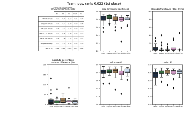
| 1 | pgs | 0.0215 | 0.81 | 5.63 | 18.58 | 0.82 | 0.79 |
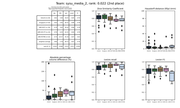
| 2 | sysu_media_2 | 0.0220 | 0.80 | 5.76 | 28.73 | 0.87 | 0.76 |
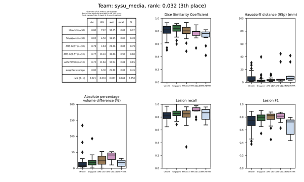
| 3 | sysu_media | 0.0320 | 0.80 | 6.30 | 21.88 | 0.84 | 0.76 |
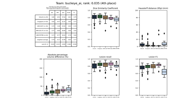
| 4 | buckeye_ai | 0.0345 | 0.79 | 6.17 | 22.99 | 0.83 | 0.77 |
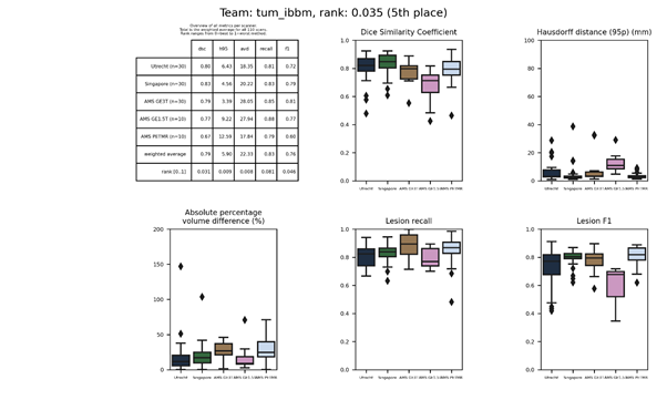
| 5 | tum_ibbm | 0.0349 | 0.79 | 5.90 | 22.33 | 0.83 | 0.76 |
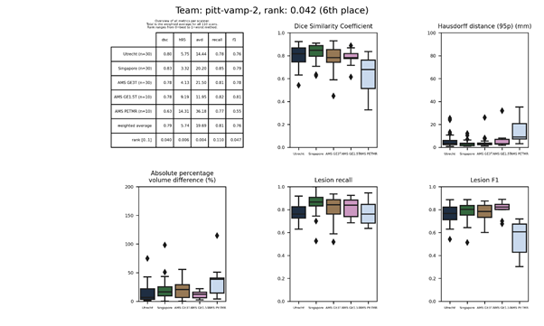
| 6 | pitt-vamp-2 | 0.0415 | 0.79 | 5.74 | 19.69 | 0.81 | 0.76 |
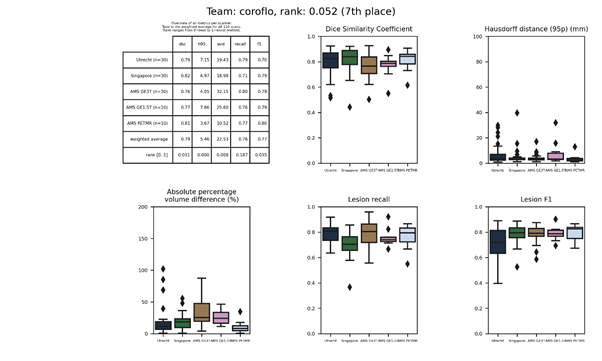
| 7 | coroflo | 0.0520 | 0.79 | 5.46 | 22.53 | 0.76 | 0.77 |
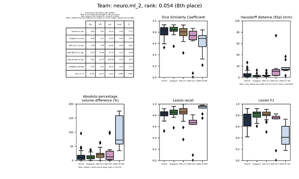
| 8 | neuro.ml_2 | 0.0541 | 0.78 | 6.33 | 30.63 | 0.82 | 0.73 |
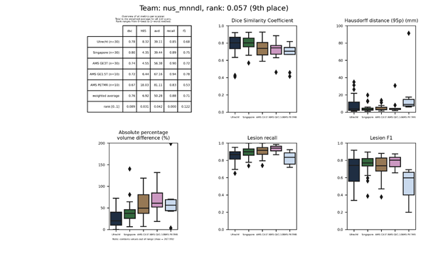
| 9 | nus_mnndl | 0.0568 | 0.76 | 6.92 | 50.28 | 0.88 | 0.71 |
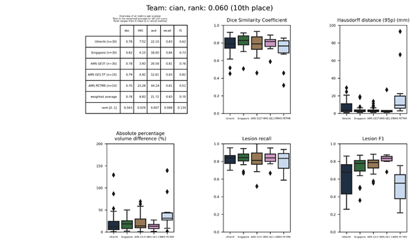
| 10 | cian | 0.0602 | 0.78 | 6.82 | 21.72 | 0.83 | 0.70 |
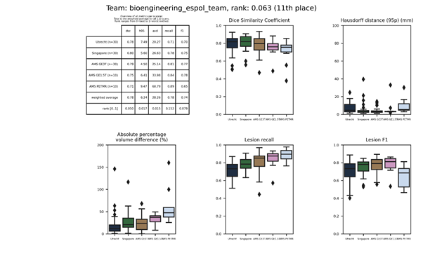
| 11 | bioengineering_espol_team | 0.0625 | 0.78 | 6.24 | 28.26 | 0.78 | 0.74 |
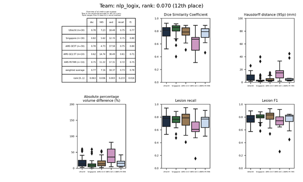
| 12 | nlp_logix | 0.0704 | 0.77 | 7.16 | 18.37 | 0.73 | 0.78 |
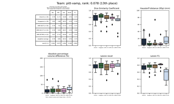
| 13 | pitt-vamp | 0.0780 | 0.79 | 8.85 | 19.53 | 0.76 | 0.73 |
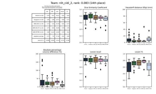
| 14 | nih_cidi_2 | 0.0833 | 0.75 | 7.35 | 27.26 | 0.81 | 0.69 |
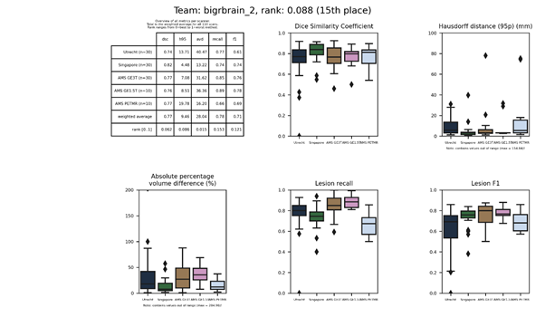
| 15 | bigrbrain_2 | 0.0876 | 0.77 | 9.46 | 28.04 | 0.78 | 0.71 |
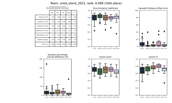
| 16 | uned_stand_2021 | 0.0890 | 0.79 | 6.37 | 17.56 | 0.69 | 0.73 |
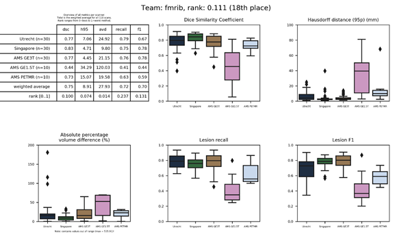
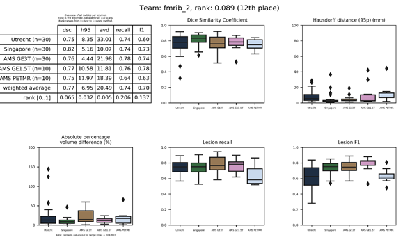
| 17 | fmrib-truenet_2 | 0.0917 | 0.77 | 6.95 | 20.49 | 0.74 | 0.70 |
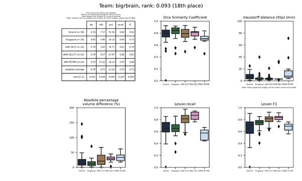
| 18 | bigrbrain | 0.0934 | 0.78 | 6.75 | 23.24 | 0.70 | 0.73 |
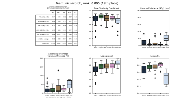
| 19 | nic-vicorob | 0.0954 | 0.77 | 8.28 | 28.54 | 0.75 | 0.71 |
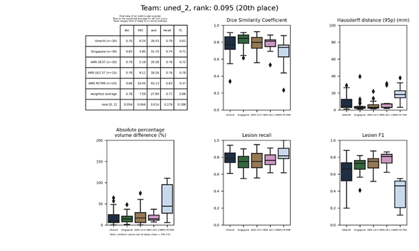
| 20 | uned_2 | 0.0954 | 0.78 | 7.59 | 27.69 | 0.77 | 0.66 |
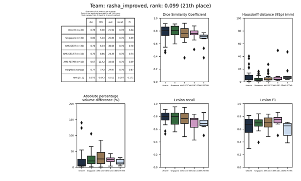
| 21 | rasha_improved | 0.0991 | 0.77 | 7.42 | 24.97 | 0.76 | 0.67 |
| 22 | wta | 0.1033 | 0.78 | 6.78 | 16.20 | 0.66 | 0.73 |
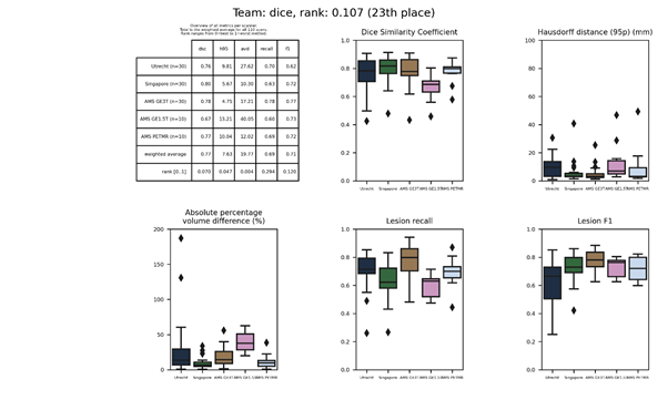
| 23 | dice | 0.1070 | 0.77 | 7.63 | 19.77 | 0.69 | 0.71 |
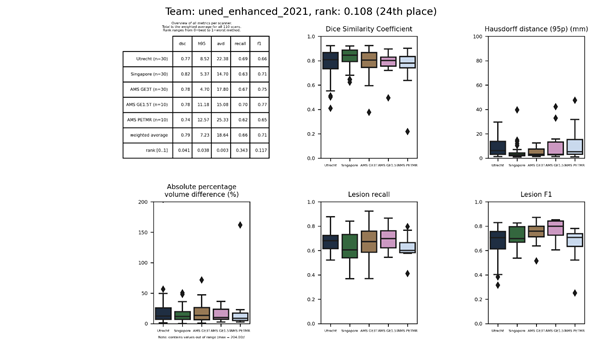
| 24 | uned_enhanced_2021 | 0.1085 | 0.79 | 7.23 | 18.64 | 0.66 | 0.71 |
| 25 | fmrib-truenet | 0.1139 | 0.75 | 8.91 | 27.93 | 0.72 | 0.70 |
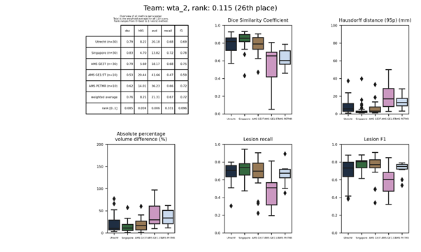
| 26 | wta_2 | 0.1154 | 0.76 | 8.21 | 21.31 | 0.67 | 0.72 |
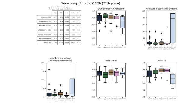
| 27 | misp_2 | 0.1201 | 0.78 | 11.10 | 19.71 | 0.68 | 0.71 |
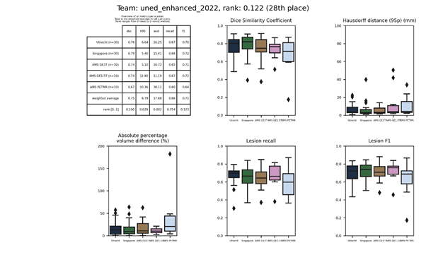
| 28 | uned_enhanced_2022 | 0.1215 | 0.75 | 6.79 | 17.68 | 0.66 | 0.71 |
| 29 | acunet_2-2 | 0.1369 | 0.71 | 8.34 | 22.58 | 0.69 | 0.70 |
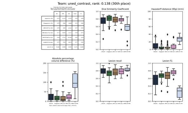
| 30 | uned_contrast | 0.1383 | 0.75 | 9.90 | 44.33 | 0.77 | 0.60 |
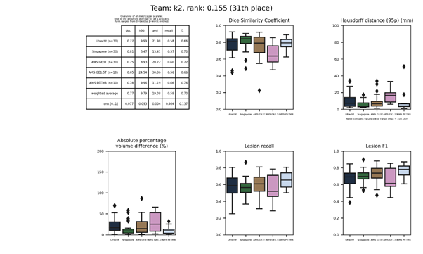
| 31 | k2 | 0.1549 | 0.77 | 9.79 | 19.08 | 0.59 | 0.70 |
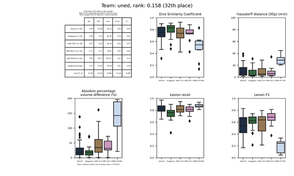
| 32 | uned | 0.1581 | 0.73 | 11.04 | 55.84 | 0.81 | 0.54 |
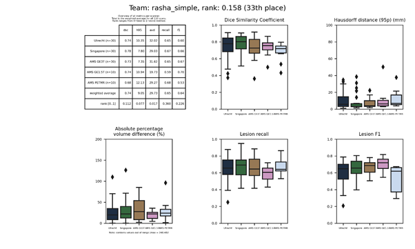
| 33 | rasha_simple | 0.1584 | 0.74 | 9.05 | 29.73 | 0.65 | 0.64 |
| 34 | acunet_2-4 | 0.1662 | 0.69 | 10.30 | 26.14 | 0.63 | 0.71 |
| 35 | acunet_2-1 | 0.1718 | 0.69 | 8.96 | 28.99 | 0.65 | 0.65 |
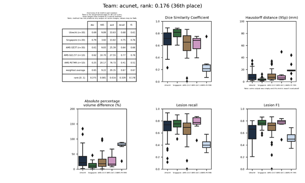
| 36 | acunet | 0.1758 | 0.65 | 9.22 | 29.35 | 0.67 | 0.67 |
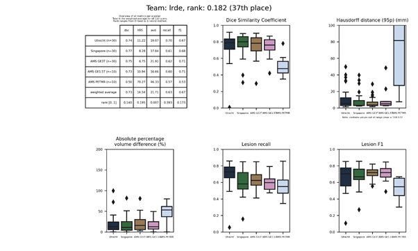
| 37 | lrde | 0.1818 | 0.73 | 14.54 | 21.71 | 0.63 | 0.67 |
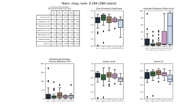
| 38 | misp | 0.1842 | 0.72 | 14.88 | 21.36 | 0.63 | 0.68 |
| 39 | acunet_2-3 | 0.2051 | 0.66 | 10.31 | 28.40 | 0.58 | 0.67 |
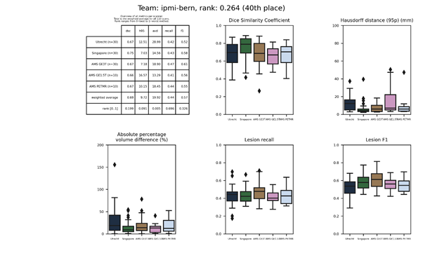
| 40 | ipmi-bern | 0.2635 | 0.69 | 9.72 | 19.92 | 0.44 | 0.57 |
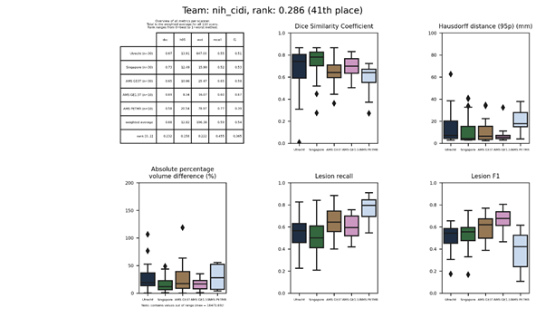
| 41 | nih_cidi | 0.2862 | 0.68 | 12.82 | 196.38 | 0.59 | 0.54 |
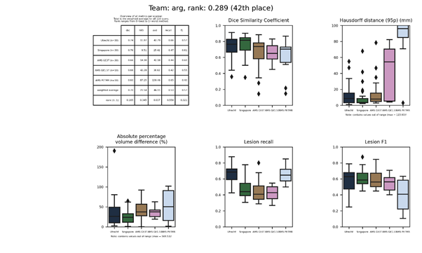
| 42 | arg | 0.2894 | 0.70 | 21.54 | 46.11 | 0.53 | 0.57 |
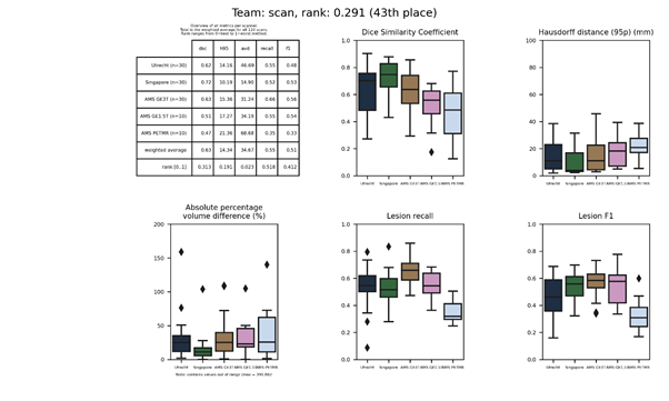
| 43 | scan | 0.2914 | 0.63 | 14.34 | 34.67 | 0.55 | 0.51 |
| 44 | tig 2 | 0.3055 | 0.68 | 17.48 | 39.07 | 0.54 | 0.46 |
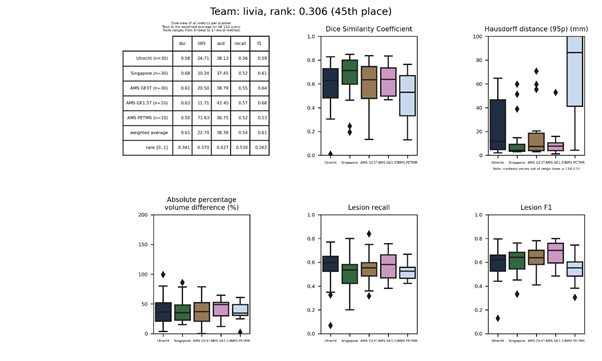
| 45 | livia | 0.3060 | 0.61 | 22.70 | 38.39 | 0.54 | 0.61 |
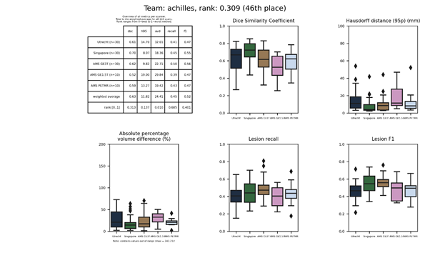
| 46 | achilles | 0.3092 | 0.63 | 11.82 | 24.41 | 0.45 | 0.52 |
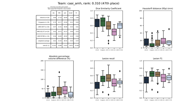
| 47 | caai_amh | 0.3101 | 0.62 | 15.03 | 28.54 | 0.45 | 0.57 |
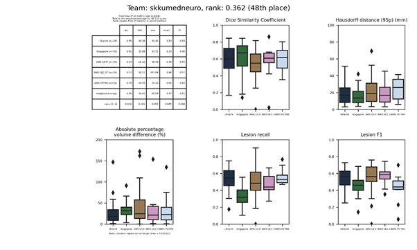
| 48 | skkumedneuro | 0.3616 | 0.58 | 19.02 | 58.54 | 0.47 | 0.51 |
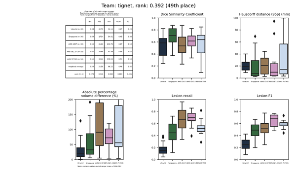
| 49 | tignet | 0.3921 | 0.59 | 21.58 | 86.22 | 0.46 | 0.45 |
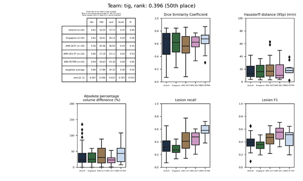
| 50 | tig | 0.3963 | 0.60 | 17.86 | 34.34 | 0.38 | 0.42 |
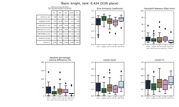
| 51 | knight | 0.4239 | 0.70 | 17.03 | 39.99 | 0.25 | 0.35 |
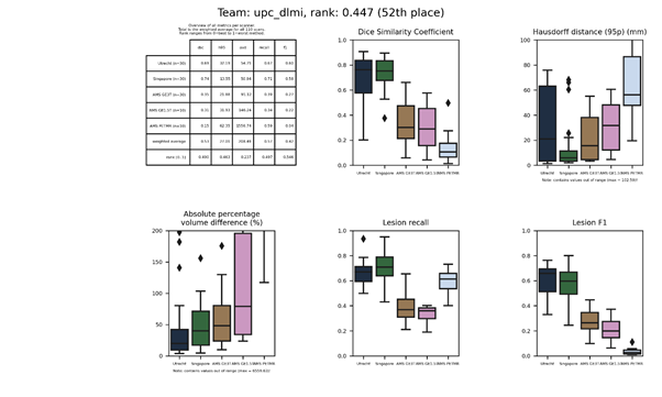
| 52 | upc_dlmi | 0.4466 | 0.53 | 27.01 | 208.49 | 0.57 | 0.42 |
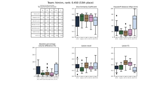
| 53 | himinn | 0.4505 | 0.62 | 24.49 | 44.19 | 0.33 | 0.36 |
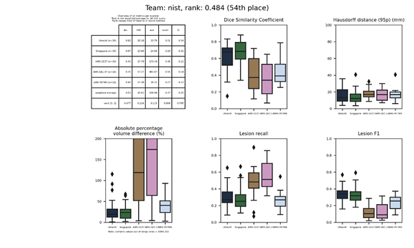
| 54 | nist | 0.4836 | 0.53 | 15.91 | 109.98 | 0.37 | 0.25 |
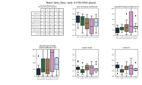
| 55 | text_class | 0.5782 | 0.50 | 28.23 | 146.64 | 0.27 | 0.29 |
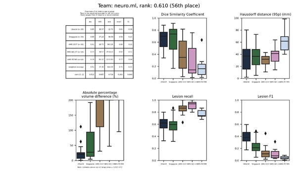
| 56 | neuro.ml | 0.6099 | 0.51 | 37.36 | 614.05 | 0.71 | 0.21 |
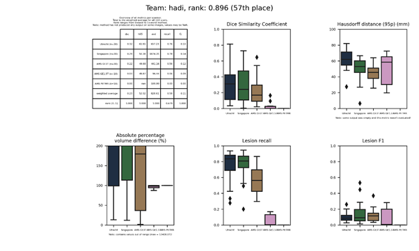
| 57 | hadi | 0.8957 | 0.23 | 52.02 | 828.61 | 0.58 | 0.11 |
Evaluation
Evaluation will be done according to the following metrics:
- Dice
- Hausdorff distance (modified, 95th percentile)
- Average volume difference (in percentage)
- Sensitivity for individual lesions (in percentage)
- F1-score for individual lesions
Individual lesions are defined as 3D connected components. The full source code that will be used for evaluation can be found here: evaluation.py.
Ranking
Each metric is averaged over all test scans. For each metric, the participating teams are sorted from best to worst. The best team receives a rank of 0 and the worst team a rank of 1; all other teams are ranked (0,1) relative to their performance within the range of that metric. Finally, the five ranks are averaged into the overall rank that is used for the Results.
For example: the best team A has a DSC of 80 and the worst team B a DSC of 60. In the ranking: A=0.00 and B=1.00. Another team C has a DSC of 78, which is then ranked at 1.0 - (78 - 60) / (80 - 60) = 0.10. The actual Python code to compute this is:
import pandas


    def getRankingHigherIsBetter(df, metric):

      return 1.0 - getRankingLowerIsBetter(df, metric)


    def getRankingLowerIsBetter(df, metric):

      rank = df.groupby('team')[metric].mean()


      lowest = rank.min()

      highest = rank.max()


      return (rank - lowest) / (highest - lowest)


    # Pandas DataFrame containing the results for each team for each


    # test
    image

    df = loadResultData()

    rankDsc    = getRankingHigherIsBetter(df, 'dsc')

    rankH95    = getRankingLowerIsBetter(df, 'h95')

    rankAvd    = getRankingLowerIsBetter(df, 'avd')

    rankRecall = getRankingHigherIsBetter(df, 'recall')

    rankF1     = getRankingHigherIsBetter(df, 'f1')


    finalRank = (rankDsc + rankH95 + rankAvd + rankRecall + rankF1) / 5
Organizers
This challenge is organized as a joint effort of the UMC Utrecht, VU Amsterdam, and NUHS Singapore.
Hugo J. Kuijf - Main organizer
Image Sciences Institute
UMC Utrecht, the Netherlands
Geert Jan Biessels - Scientific advisory board
Brain Center Rudolf Magnus
UMC Utrecht, the Netherlands
Max A. Viergever - Scientific advisory board
Image Sciences Institute
UMC Utrecht, the Netherlands
Christopher Chen - Scientific advisory board
Memory Aging and Cognition Center
NUHS, Singapore
Wiesje van der Flier - Scientific advisory board
Alzheimer Center
VU Amsterdam, the Netherlands
Frederik Barkhof - Scientific advisory board
Image Analysis Centre
VU Amsterdam, the Netherlands
Jeroen de Bresser - Medical advisory board
Department of Radiology
UMC Utrecht, the Netherlands
Matthijs Biesbroek - Medical advisory board
Brain Center Rudolf Magnus
UMC Utrecht, the Netherlands
Rutger Heinen - Medical advisory board
Brain Center Rudolf Magnus
UMC Utrecht, the Netherlands
Teams
Below are the results of every submitted method on the test data.
achilles
A neural network similar to HighResNet and DeepLab v3, utilizing atrous (dilated) convolutions, atrous spatial pyramid pooling, and residual connections. The network is trained only on the FLAIR images, taking random 713 sized patches, and applying scaling and rotation augmentations.
Full description of this method.
Docker
container of this method.
acunet
An Asymmetric Compact U-Net (ACU-Net) implementation that is: asymmetric (smaller decoder compared to encoder), compact (fewer channels), and uses depthwise convolutional layers.
Full description of this method.
arg
An ensemble of ten ResNet models, which are trained sequentially. After training the first model, a cosine similarity metric was added to the loss of the next models. The aim is to have each layer learn different features in comparison to the previously trained models.
bigrbrain
A convolutional neural network with a 3D U-Net architecture, followed by a posterior-CRF to improve the results of the CNN.
Description of the method.
Docker
container of this method.
An update of this method is available: bigrbrain 2.
bigrbrain 2
A convolutional neural network with a 3D U-Net architecture, followed by a posterior-CRF to improve the results of the CNN.
Description of this method.
Docker
container of this method.
This method is an update of bigrbrain.
bioengineering_espol_team
Similar to sysu_media, but with less layers in the U-net and no ensemble.
Description of the method.
Docker container.
Full paper.
buckeye_ai
A “brain atlas guided attention U-net” implementation that consists of two separate encoding-decoding paths: one for the image itself and one for an aligned MNI152 atlas. Multi-input attention modules (MAM) and attention fusion modules (AFM) are used to combine both paths.
Description of the method.
Arxiv publication.
Full text publication.
Docker
container.
caai_amh
A modified version of sysu_media, which is transfer learned on a private data set with FLAIR images of MS patients (not the challenge data set). Modifications include adding neighbouring slices as channels, more dropout, and no ensemble.
Full description of the method.
cian
A network based on multi-dimensional gated recurrent units (MD-GRU) was trained on 3D patches using data augmentation techniques including random deformation, rotation and scaling.
Presentation of this method.
Full description of this method.
coroflo
Docker container of this method.
dice
An ensemble of five neural networks similar to No New-Net, each trained on a different subset of the training data.
Full description of this method.
fmrib-truenet
A “triplanar U-Net ensemble network (TrUE-Net)”, combining three U-nets that each process one of the three main orthogonal planes.
Full description of this method.
fmrib-truenet 2
This method is an update of fmrib-truenet. It adds new data preparation steps and as post-processing applies a white matter mask.
Full description of the method.
Source code.
Publication.
Docker container.
hadi
A random forest classifier trained on multi-modal image features. These include intensities, gradient, and Hessian features of the original images, after smoothing, and of generated super-voxels.
Presentation of this method.
Full description of this method.
Docker container of this method.
himinn
An unsupervised 3D segmentation autoencoder (SegAE) using fully convolutional layers on three scales. The network is optimized based on Cosine proximity; and outputs four channels for GM, WM, CSF, and WMH separately.
Full description of this method.
ipmi-bern
A two-stage approach that uses fully convolutional neural networks to first extract the brain from the images and second identifies WMH within the brain. Both stages implement long and short skip connections. The second stage produces output at three different scales. Data augmentation was applied, including rotations and mirroring.
Presentation of this method.
Full description of this method.
Docker
container of this method.
k2
A 2D fully convolutional neural network with an architecture similar to U-Net. A number of models were trained for the whole dataset, as well as for each individual scanner. During application, first the type of scanner was predicted and next that specific model was applied together with the model trained on all data.
Presentation of this method.
Full description of this method.
Docker container of this method.
knight
A voxel-wise logistic regression model that is fitted independently for each voxel in the FLAIR image. Images were transformed to the MNI-152 standard space for training and at test time the parameter maps were warped to the subject space.
Presentation of this method.
Full description of this method.
Docker
container of this method.
livia
lrde
A modification of the pre-trained 16-layer VGG network, where the FLAIR, T1, and a high-pass filtered FLAIR are used as multi-channel input. The VGG network had its fully connected layers replaced by a number of convolutional layers.
Presentation of this method.
Full description of this method.
misp
A 3D convolutional neural network with 18 layers using patches of 27×27×9 voxels. The first eight layers were trained separately for the FLAIR and T1 images and had skip-connections.
Presentation of this method.
Full description of this method.
Docker container of this method.
An updated submission is available: misp 2.
misp 2
This submission is an update of misp Description
neuro.ml
A neural network using the DeepMedic architecture, having two parallel branches that process the images at two different scales. The network used 3D patches, which were sampled such that 60 % of the patches contained a WMH.
Full description of this method.
An updated submission is available: neuro.ml 2.
neuro.ml 2
This submission is an update of neuro.ml. Description.
nic-vicorob
A 10-layer 3D convolutional neural network architecture previously used to segment multiple sclerosis lesions. A cascaded training procedure was employed, training two separate networks to first identify candidate lesion voxels and next to reduce false positive detections. A third network re-trains the last fully connected layer to perform WMH segmentation.
Presentation of this method.
Full description of this method.
Docker
container of this method.
nih_cidi
A fully convolutional neural network modified from the U-Net architecture was used to segment WMH on the FLAIR images. Next, another network was trained to segment the white matter from T1 images, and the segmented white matter mask is applied to remove false positives from the WMH segmentation results. The original U-Net architecture was trimmed to keep only three pooling layers.
Presentation of this method.
Full description of this method.
Docker
container of this method.
An updated submission is available: nih_cidi 2.
nih_cidi 2
This submission is an update of nih_cidi Description Full
text
nist
A random decision forest classifier trained on location and intensity features.
Presentation of this method.
Full description of this method.
Docker container of this method.
nlp_logix
A multiscale deep neural network similar to Ghafoorian et al., with some minor modifications and no spatial features. The network was trained in ten folds and the three best performing checkpoints on the training data were selected. These were applied on the test set and the results averaged.
Presentation of this method.
Full description of this method.
Docker
container of this method.
nus_mnndl
An ensemble of ten 3D U-Nets, where the encoder is pre-trained from the UK Biobank brain age prediction and the decoder is optimized using deep supervision
Full description of method.
GitHub source codes.
Docker
container.
pitt-vamp
A convolutional domain adversarial neural network (CDANN) connected to the lower layers of a common U-Net, trained only on FLAIR images.
Full description of the method.
Docker
container.
pitt-vamp 2
This method is an update of pitt-vamp and added mixup to the training procedure.
Description of the method.
Docker
container.
pgs
An ensemble of 5 randomly initialized 2D U-Net models trained on augmented data. In the decoding path, max-pooled versions of the original images are reintroduced to highlight WMH information. During inference, original images flipped versions (flipped along the x-axis, y-axis, and both) processed by the five ensembles and aggregated.
Description of the method.
Docker container of this method.
Journal
paper of the method.
rasha_improved
This is an improved version of rasha_simple. It is meant to show the impact of data augmentation with respect to the simple version.
rasha_simple
This is a simple U-Net model that can be compared to rasha_improved, of which the latter has more extensive data augmentation.
scan
A densely connected convolutional network using dilated convolutions. In each dense block, the output is concatenated to the input before passing it to the next layer. Two classifiers were trained: one to apply brain extraction and the second to find lesions within the extracted brain.
Presentation of this method.
Full description of this method.
skkumedneuro
An intensity-based thresholding method with region growing approach to segment periventricular and deep WMH separately, and two random forest classifiers for false positive reduction. Per imaging modality, 19 texture and 100 “multi-layer” features were computed. The “multi-layer” features were computed using a feed-forward convolutional network with fixed filters (e.g. averaging, Gaussian, Laplacian); consisting of two convolutional, two max-pooling, and one fully connected layer.
Presentation of this method.
Full description of this method.
Docker
container of this method.
sysu_media
A fully convolutional neural network similar to U-Net. An ensemble of three networks was trained with different initializations. Data normalization and augmentation was applied. To remove false positive detections, WMH in the first and last ⅛th slices was removed.
Presentation of this method.
Full description of this method.
Docker
container of this method.
An updated submission is available: sysu_media 2.
sysu_media 2
This submission is an update of sysu_media. Description.
text_class
A random forest classifier trained primarily on texture features. Features include local binary pattern, structural and morphological gradients, and image intensities.
Presentation of this method.
Full description of this method.
Docker
container of this method.
tig
A three-level Gaussian mixture model, slightly adapted from Sudre et al. The model is iteratively modified and evaluated, until it converges. After that, candidate WMH is selected and possible false positives are pruned based on their location.
Presentation of this method.
Full description of this method.
An updated submission is available: tig 2.
tig 2
This submission is an update of tig. Description (PDF).
tignet
A neural network with the HighResNet architecture. The network was trained on 2,660 images segmented using the method of team tig.
Presentation of this method.
Full description of this method.
Docker
container of this method.
tum_ibbm
This method applies subject-wise unsupervised domain adaptation to a neural network based on previous methods (sysu_media and sysu_media-2).
uned
An attention gate U-net with three levels, trained on FLAIR and T1 using data augmentation.
Full description of this method.
Docker container.
uned 2
This is an updated version of uned.
uned_contrast
A modified version of uned.
uned_enhanced-2021
Same as uned_stand-2021, but a non-linear contrast enhancement is applied to the FLAIR images.
uned_enhanced-2022
This submission is an update of uned_enhanced-2021.
uned_stand-2021
An attention gate U-net with three levels, trained on FLAIR and T1 using data augmentation. This method is an update of uned.
upc_dlmi
A neural network modified from the V-Net architecture. An additional network with convolutional layers is trained on upsampled images and then concatenated with the output of the V-Net.
Presentation of this method.
Full description of this method.
Docker container of this method.
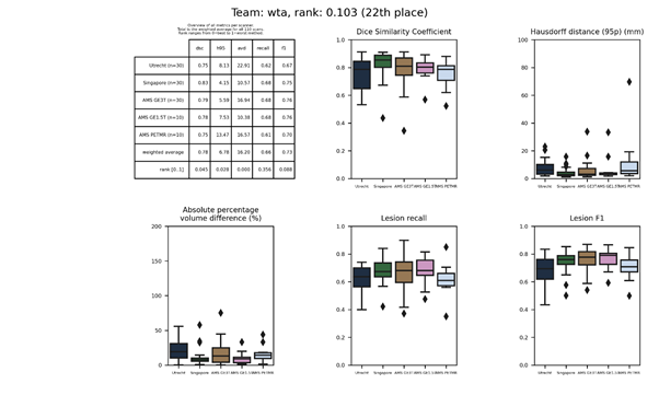
wta
An ensemble of five Hybrid Attention – Densely Connected Networks, based on the U-Net architecture, with skip-connections at the central layers and a hybrid attention block in the decoding path.
Description of the method.
Docker container of this method.
wta 2
This is an updated method of wta.